leftRightCharlotte = moveXY wiggle 0 charlotte charlotte = importBitmap "../Media/charlotte.bmp" |
|
We have all seen a lot of wonderful looking computer graphics, and many of us have spent time playing video games or watching our kids (or their kids) play them. It is clear that computer graphics, especially interactive graphics, is an incredibly expressive medium, with potential beyond our current imagination.
Affordable personal computers are capable of very impressive 2D animation and multi-media. Interactive 3D graphics is already available, and soon it will be standard for new personal computers. Thus, the raw materials for creating and sharing interactive graphics are in reach of all of us.
That's the good news.
The bad news is that very few people are able to create their own interactive graphics, and so what might otherwise be a widely shared medium of communication is instead a tool for specialists. The problem is that there are too many low-level details that have to do not with the desired content -- e.g., shapes, appearance and behavior -- but rather how to get a computer to present the content. For instance, behaviors like motion and growth are generally gradual, continuous phenomena. Moreover, many such behaviors go on simultaneously. Computers, on the other hand, cannot directly accommodate either of these basic properties, because they do their work in discrete steps rather than continuously, and they only do one thing at a time. Graphics programmers have to spend much of their effort bridging the gap between what an animation is and how to present it on a computer.
One approach to solving this problem is to avoid programming altogether, and instead use a visual authoring tool. These tools are becoming quite powerful and reasonably easy to use, but they are not nearly as flexible as programming, especially for interactive content, in which decisions have to be made dynamically.
If programming is necessary for the creation of interactive content, but the kind of programming used to make such content today is unsuitable for most of the potential authors, then we need to move toward a different form of programming. This form must give the author complete freedom of expression to say what an animation is, while invisibly handling details of discrete, sequential presentation. In other words, this form must be declarative ("what to be") rather than imperative ("how to do").
This article presents one approach to declarative programming of interactive content, as realized in a prototype system called Fran, for "Functional reactive animation" [Elliott and Hudak 1997, Elliott 1997]. Fran is a high level vocabulary that allows one to describe the essential nature of an animated model, while omitting details of presentation. Moreover, because this vocabulary is embedded in a modern functional programming language (Haskell), the animation models thus described are reusable and composable in powerful ways.
I do not assume familiarity with Haskell, and have tried to make this article mostly self-contained. This is hard to do well, and requires that you take some of the details on faith for now. See [Thompson 1996], [Bird and Wadler 1987] and [Hudak and Fasel 1992] for introductions to functional programming in general and Haskell in particular and [Hudak et al 1992] for reference. Another Haskell resource is haskell.org on the web.
Fran is currently available, with all source code, as part of the Hugs 1.4 implementation of Haskell for Windows 95 and Windows NT, which is freely available [Yale and Nottingham 1998]. Newer versions of Fran may be found at http://conal.net/fran/.
This article contains several animation examples to illustrate our declarative approach to animation. Executable source code appears as lines of text in this font. There are three ways to experience this article, with increasing levels of immersion.
We'll start with a very simple animation, called leftRightCharlotte, of Charlotte moving from side to side.
leftRightCharlotte = moveXY wiggle 0 charlotte charlotte = importBitmap "../Media/charlotte.bmp" |
|
The first line defines a value called leftRightCharlotte to be the result of applying the function moveXY to three arguments. (In most other programming languages, you would instead say something like "moveXY(wiggle,0,charlotte)".)
The function moveXY takes x and y values and an image, and produces an image moved horizontally by x and vertically by y. All values may be animated. In this example, the x value is given by a predefined smoothly animated number called wiggle. Wiggle starts out at zero, increases to one, decreases back past zero to negative one, and then increases to zero again, all in the course of two seconds, and then it repeats, forever.
The second line defines charlotte by importing a bitmap file, making it available for use on the first line as the second argument to moveXY.
Although this first example is not exactly a masterpiece, it is a complete animation program in just two short lines!
Similarly, we can define an animation of Patrick moving up and down:
upDownPat = moveXY 0 waggle pat pat = importBitmap "../Media/pat.bmp" |
|
To get the vertical movement, we use a nonzero value for the second argument to moveXY. Rather than using wiggle, we use waggle, which is defined to be just like wiggle, but delayed by a half second.
Next we move on to a simple animation that my daughter Becky and I cooked up one evening. This one combines the two previous examples.
charlottePatDance = leftRightCharlotte `over` upDownPat |
|
The over operation glues two given animations together, yielding a single animation, with the first one being over the second. Because we used waggle for upDownPat, in this new combined animation Pat is at the center when Charlotte is at her extremes and vice versa.
To provide a contrast, here is a very rough sketch of the steps one usually goes through to program an animation.
These steps are usually carried out with lots of tedious, low-level code that you have to write yourself.
Most of this work is not about what the animation is, but how to present it. In contrast, Fran programs are only about what the animation is.
"Composition" is the principle of putting together simpler things to make more complex things, then putting these together to make even more complex things, and so on. This "building block" principle is crucial for making even moderately complicated constructions; without it, the complexity quickly becomes unmanageable.
The examples above illustrate composition. We first built leftRightCharlotte out of charlotte, wiggle and moveXY; then we built upDownPat out of pat, moveXY and waggle; and finally we built charlottePatDance out of leftRightCharlotte and upDownPat. A crucial point here is that when we make something out of building blocks, the result is a new building block in itself, and we can forget about how it was constructed.
There is a still more powerful version of composition, based on defining functions. For example, let us now define a new function called hvDance (for horizontally and vertical dance), that can combine any two images, in the way that charlottePatDance combines charlotte and pat:
  hvDance im1 im2 =
    moveXY wiggle 0 im1  `over`
    moveXY 0 waggle im2
|
Now we can give a new definition for our dancing couple that gives exactly the same animation:
charlottePatDance = hvDance charlotte pat |
Having defined this generalized dance animation, we can go on to more exotic compositions. For example, we can take an animation produced by hvDance, shrink it, and put the result back into hvDance twice to make it dance with itself. The result is pleasantly surprising.
 charlottePatDoubleDance = hvDance aSmall aSmall
   where
    aSmall = stretch 0.5 charlottePatDance
|
|
This example gives you a hint of how powerful it is to be able to define new animation functions. The possibilities are limitless, so I encourage you to apply your imagination and try out more variations. Here are a few more, just to give you ideas.
We could try charlottePatDance, stretched by a wiggly amount. To prevent negative scaling, we take the absolute value of wiggle.
dance1 = stretch (abs wiggle) charlottePatDance |
|
Next, use hvDance again, but give it wiggly-sized charlotte and pat. This time, we haven't prevented negative scaling. For visual balance, we use wiggle and waggle.
 dance2 = hvDance (stretch wiggle charlotte)
                  (stretch waggle pat)
|
|
Next, put Pat in orbit around a growing and shrinking Charlotte. To get a circular motion, we use the moveXY function, with wiggle for x and waggle for y.
patOrbitsCharlotte = stretch wiggle charlotte `over` moveXY wiggle waggle pat |
|
By the way, if you remember your high school trigonometry, you may have surmised that wiggle and waggle are related to sine and cosine. In fact, they are defined very simply, as follows:
waggle = cos (pi * time) wiggle = sin (pi * time) |
The animated number called time is a commonly used "seed" for animations and has the value t at time t. Thus, for instance, the value of wiggle at time t is equal to sin (p t).
In the previous examples, the positions of animations are specified directly. For instance, the definition of leftRightCharlotte says that Charlotte's horizontal position is wiggle.
In our physical universe, objects move as a consequence of forces. As Newton explained, force leads to acceleration, acceleration to velocity, and velocity to position. With computer animation, an author has the freedom to ignore the laws of our universe. However, since animations are usually intended to be viewed by and interacted with by inhabitants of our own universe, they are often made to look and feel real by emulating the Newtonian laws or simplifications and variations on them.
The key idea underlying Newton's laws and their variations is the notion of an instantaneous rate of change. Fran makes this notion available in animation programs. As a first, very simple, illustration of rate-based animation, we can make Becky move from the left edge of our viewing window, toward the right, at a rate of one distance unit per second.
 velBecky u = moveXY x 0 becky
   where
     x = -1 + atRate 1 u
|
|
The local definition of x here (introduced as a "where clause"), follows a style you will see in the following few definitions. To express an animated value that starts out with a value x0 and grows at a rate of r, one says "x0 + atRate r u". Here u is a "user", which is a Fran value that contains all user input and display update events. Rate-based animations require a user argument in order to give atRate a way of knowing when to start and how precisely to calculate value from rate. Unlike the previous examples, this one can be displayed with the function displayU, so to see this example, type "displayU velBecky". We will see other uses for this user argument below.
In the velBecky example, Becky has a constant velocity, but with only a little more effort, we can give Becky a constant acceleration instead, by providing a constant value for the rate of change of the velocity.
 accelBecky u = moveXY x 0 becky
   where
     x = -1 + atRate v u
     v =  0 + atRate 1 u
|
|
In the definition of v, the "0 +" is unnecessary, but emphasizes that the initial velocity is zero.
The notion of "rate" is useful not just in one dimension, but in two and three dimensions as well. In the next example, we will control Becky's two-dimensional velocity with the mouse. When you hold the mouse cursor at the center of the view window, Becky will stay still. As you move away from the center, imagine an arrow from the window's center to the mouse cursor. Becky will be moving in that direction and her speed will be equal to the arrow's length. This kind of imaginary arrow is referred to as a vector, and is the type of quantity that a two- or three-dimensional offset, velocity or acceleration is. In 2D, a vector can be thought of as having horizontal and vertical (X and Y) components, or as having a magnitude (length) and direction.
 mouseVelBecky u = move offset becky
   where
    offset = atRate vel u
    vel    = mouseMotion u
|
|
This time, we're using the function move, a variant of moveXY that takes a 2D offset vector. (If a vector v is x units horizontally and y units vertically, then "move v im" is equivalent to "moveXY x y im"). The offset vector starts out as the zero vector, and grows at a rate equal to mouseMotion, which is the offset of the mouse cursor relative to the origin of 2D space (which we see at in the center of the view window).
In the real world, the position of an object may affect its speed or acceleration. In the next example, Becky is chasing the mouse cursor. The further away he is, the faster she moves.
 beckyChaseMouse u = move offset becky
   where
    offset = atRate vel u
    vel    = mouseMotion u - offset
|
|
The only difference from the previous example is that the velocity is determined by where the mouse cursor is relative to Becky's own position, as indicated by the vector subtraction.
Just for fun, we can generalize the beckyChaseMouse function in the same way that hvDance generalized charlottePatDance in an earlier example.
 chaseMouse im u = move offset im
   where
    offset = atRate vel u
    vel    = mouseMotion u - offset
|
Then "chaseMouse becky" is equivalent to beckyChaseMouse, as you can verify by typing the following to the Hugs prompt:
displayU (chaseMouse becky)
For more fun, try the same, but replacing becky by some of the animations that appear earlier in this article, e.g., leftRightCharlotte, charlottePatDance, and patOrbitsCharlotte.
danceChase u = chaseMouse (stretch 0.5 charlottePatDance) u |
|
Next let's make a chasing animation that acts like it is attached to the mouse cursor by a spring. The definition is very similar to beckyChaseMouse. This time, however, the rate is itself changing at a rate we call accel (for acceleration). This acceleration is defined like the velocity was in the previous example, but this time we also add some drag that tends to slow down Becky by adding some acceleration in the direction opposite to her movement. (Increasing or decreasing the "drag factor" of 0.5 below creates more or less drag.)
 springDragBecky u = move offset becky
   where
    offset = atRate vel u
    vel    = atRate accel u
    accel  = (mouseMotion u - offset) - 0.5 *^ vel
|
|
The operator *^ multiplies a number by a vector, yielding a new vector that has the same direction as the given one but a scaled magnitude.
As usual, these declarative animation programs are simple because they say what the motion is, in high level, continuous terms, without struggling to accommodate the discreteness of the computer used to present them. In contrast, imperative animation programs must explicitly simulate rate-based animation by making lots of little discrete steps, accumulating approximations to the continuously varying forces, accelerations, and velocities, in order to approximate motion. Doing an accurate and efficient job of all this approximation work is a very tricky task. With a system like Fran, the author just describes the continuous motion in terms of continuously varying rates, and trusts to Fran to do a good job with the approximation. (Not good enough to fly a real airplane or control dangerous machinery, but good enough for a pleasant and effective illustration or game.)
Operations like over and move support the principle of composition in space. Composition in time is equally valuable. As a first example, let's define an orbiting animation, and then combine it with a version of itself delayed by one second.
 orbitAndLater = orbit `over` later 1 orbit
   where
    orbit = moveXY wiggle waggle jake
|
|
Instead of delaying, we may want to speed it up.
 orbitAndFaster = orbit `over` faster 2 orbit
   where
    orbit = move wiggle waggle jake
|
|
We can even delay or slow down animations involving user input. In the following example, one Jake tracks the mouse cursor, while the other follows the same path, but delayed by one second.
 followMouseAndDelay u =
  follow `over` later 1 follow
   where
    follow = move (mouseMotion u) jake
|
|
Next let's build an animated sentence, following the mouse's motion path. As a preliminary step, define a function delayAnims, which takes a time delay dt and a list anims of animations, and yields an animation. Each successive member of the given animation list is delayed by the given amount after the previous member.
delayAnims dt anims = overs (zipWith later [0, dt ..] anims) |
The definition of delayAnims introduces a few new Fran elements. The Fran function overs is like over, but it applies to a list of animations rather than just two. Animations earlier in the list are placed over ones later in the list. The notation [0, dt ...] means the infinite list of numbers 0, dt, 2 dt, 3 dt, etc. Finally, the function zipWith applies a given two argument function the successive values from two given lists. We use it here to delay the first animation in anims by 0 seconds, the second by dt seconds, the third by 2 dt seconds, etc. Finally, overs combines them into a single animation.
Here is a very simple use of delayAnims.
 kids u =
   delayAnims 0.5
     (map (move (mouseMotion u))
          [jake, becky, charlotte, pat])
|
|
Next, use delayAnims, to define a function mouseTrailWords that makes animated sentences.
 trailWords motion str =
   delayAnims 1 (map moveWord (words str))
   where
     moveWord word = move motion (
                      stretch 2 (
                        withColor blue (stringIm word) ))
|
A few words of explanation are in order. The Haskell function words takes a string apart into a list of separate words. The Haskell function map takes a function (here moveWord) and a list of values (here the separated words) and makes a new list by applying the function to each member of the list. The Fran function stringIm makes a picture of a string. We define the function moveWord locally to be the result of making a picture of the given word, using the Fran function stringIm, and moving it to follow the mouse. The function delayAnims, defined above, then causes each of these mouse-following word pictures to be delayed by different amounts.
Here is one use of trailWords:
 flows u = trailWords motion
             "Time flows like a river"
   where
     motion = 0.7 *^ vector2XY (cos time)
                               (sin (2 * time))
|
|
Here is another, this time following the mouse:
 flows2 u = trailWords (mouseMotion u)
              "Time flows like a river"
|
|
The animations so far are all what might be called "non-reactive", meaning that they are always doing the same thing. A "reactive animation" is one involving discrete changes, due to events. As a very simple example, we make a circle whose color starts off red and changes to blue when the left mouse button is first pressed. (The animated figure below is made to repeat, so that you do not miss the transition, but when run, the animation really changes color only once.)
 redBlue u = buttonMonitor u `over`
             withColor c circle
   where
    c = red `untilB` lbp u -=> blue
|
|
An informal reading of the last line is that the color c is red until the user presses the left mouse button, and them becomes blue. For a more literal reading of this example, one must understand that there are really two new binary infix operators here, untilB and "-=>", which can be used separately or together. The implied parentheses are around "lbp u -=> blue". The "-=>" operator, which can be read as "handled by value" takes an event (here lbp u) and a value (here blue), and yields a new event. In this case, the new event happens when the left button is pressed, and has value blue. The untilB operator takes an animation of any type (here the color-valued constant animation red), and an event (here "lbp u -=> blue"), whose occurrence provides a new animation of the same type.
To make the previous example more interesting, let's switch between red and blue every time the left button is pressed. We accomplish this change with the help of a function cycle that takes two colors, c1 and c2, and gives an animated color that starts out as c1. When the button is pressed, it swaps c1 and c2 and repeats (using recursion).
 redBlueCycle u = buttonMonitor u `over`
                  withColor (cycle red blue u)
                            circle
   where
    cycle c1 c2 u =
     c1 `untilB` nextUser_ lbp u ==> cycle c2 c1
|
|
This time, we have used the operator "==>", which is a variant of "-=>". This new operator, which can be read as "handled with function", takes an event and a function f. It works just like "-=>", but gets event values by applying f to event values from the event given to it. In this case, the function f is our cycle function applied to just two arguments, leaving the third one (a user) to be filled in automatically ==>. The nextUser_ function is used here to turn lbp into an event whose occurrence information is a new user, corresponding to the remainder of the user u. Note that the color arguments get swapped each time "around the loop".
Just to show some more variety, let's now use three colors, and have the circle's size change smoothly.
 tricycle u =
    buttonMonitor u `over`
    withColor (cycle3 green yellow red u) (
      stretch (wiggleRange 0.5 1)
        circle )
   where
    cycle3 c1 c2 c3 u =
     c1 `untilB` nextUser_ lbp u ==>
     cycle3 c2 c3 c1
|
|
The next example is a flower that starts out in the center and moves to left or right when the left or right mouse button is pressed, returning to the center when the button is released.
 jumpFlower u = buttonMonitor u `over`
                moveXY (bSign u) 0 flower

 flower = stretch 0.4
            (importBitmap "../Media/rose medium.bmp")

 bSign u = selectLeftRight 0 (-1) 1 u
|
|
The function bSign here is defined to be negative one when the left button is down, positive one when the right button is down, and zero otherwise, thanks to selectLeftRight (defined below).
We can use bSign to control the rate of growth of an image. Below, pressing the left (or right) button causes the image to shrink (or grow) until released. Put another way, the rate of growth is 0, -1, or 1, according to bSign.
 growFlower u = buttonMonitor u `over`
                stretch (grow u) flower

 grow u = size
  where
   size = 1 + atRate rate u
   rate = bSign u
|
|
A very simple change to the grow function above causes the image to grow or shrink at a rate equal to its own size.
 growFlowerExp u = buttonMonitor u `over`
                   stretch (grow' u) flower

 grow' u = size
  where
   size = 1 + atRate rate u
   rate = bSign u * size
|
|
The function selectLeftRight, used above to define bSign is also the key ingredient in defining buttonMonitor, which we have been using to give button feedback.
 buttonMonitor u =
   moveXY 0 (- height / 2 + 0.25) (
    withColor textColor (
     stretch 2 (
     stringBIm (selectLeftRight "(press a button)" "left" "right" u))))
  where
    (width,height) = vector2XYCoords (viewSize u)
|
The function stringBIm turns an animated string into an image animation, which here gets enlarged, colored white, and moved down by a little less than half the window height.
The function selectLeftRight can itself be defined in terms of more basic functions, as follows:
 selectLeftRight none left right u =
   condB (leftButton u) (constantB left) (
     condB (rightButton u) (constantB right) (
       constantB none ))
|
We use the conditional function condB to say that if the left button is down use the left value, and otherwise, if the right button is down use the none value, and otherwise use the none. (Technical fine point: constantB, which turns constants (non-animations) into animations that never change.)
The ideas of declarative animation, as illustrated in the previous 2D examples, apply to 3D as well. The 2D operations we used above, like importBMP, moveXY, and stretch have 3D counterparts. As a first 3D example, here is a sphere:
sphere = importX "../Media/sphere2.x" |
 |
The function importX brings in a 3D model in "X file" format, as used by Microsoft's DirectX.
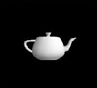
Just as easily, we can import a teapot.
teapot = stretch3 2 (importX "../Media/tpot2.x") |
|
We used stretch3, a 3D counterpart to stretch, because the imported model was too small. Now let's color our teapot and make it spin around the Z (vertical) axis.
 redSpinningPot =
   turn3 zVector3 time (
    withColorG red teapot)
|
|
Next, we can use the mouse to control the teapot's orientation. To do this, we define a function mouseTurn that turns a given geometry g around the X axis according the mouse's vertical movement, and around the Z axis according the mouse's horizontal movement scaled by pi. Then we apply mouseTurn to a green teapot.
 mouseTurn g u =
   turn3 xVector3 y (
    turn3 zVector3 (-x) g)
  where
    (x,y) = vector2XYCoords (pi *^ mouseMotion u)

 mouseSpinningPot u =
   mouseTurn (withColorG green teapot) u
|
|
We can also make teapots spin by controlling the rotation angle with the grow function, as in the growing flower examples above. First, define a function spinPot that takes (animated) color and angle and yields a colored, turning teapot:
 spinPot potColor potAngle =
   turn3 zVector3 potAngle (
    withColorG potColor teapot)
|
Then make a pot that spins one way when the left button is pressed and the other way the the right button is pressed, using the grow function defined previously and giving feedback with buttonMonitor.
 spin1 u = buttonMonitor u `over`
           renderGeometry (spinPot red (grow u))
                          defaultCamera
|
|
The renderGeometry function, used here with a convenient default camera, turns a 3D animation into a 2D one.
We'll want to make a few more spinning teapot examples, and they will all have the general form of using the button monitor and rendering with the default camera. Rather than having to write several similar definitions, let's give the pattern a name.
 withSpinner f u =
   buttonMonitor u `over`
   renderGeometry (f (grow u) u)
                  defaultCamera
|
The function withSpinner takes a function as its first argument, and applies that function to the result of the grow function applied to the user argument. With this definition, we can write spin1 more simply:
 spin1 = withSpinner spinner1
  where
    spinner1 angle u = spinPot red angle
|
As a second example of using withSpinner, let's make the color vary in hue and use the value from grow to determine the time-varying speed of rotation, so that the mouse buttons cause the turning to accelerate and decelarate.
 spin2 = withSpinner spinner2
  where
    spinner2 potAngleSpeed u =
      spinPot (colorHSL time 0.5 0.5)
              (atRate potAngleSpeed u)
|
|
In addition to visible geometry, we can add lights to a 3D model. In this next example, we combine of a white sphere, which is visible but does not emit light, and a "point light source", which is invisible but emits light. We color the sphere/light pair white, shrink it, and give it motion. For convenience, we express the motion path in terms of "spherical coordinates", saying that the distance from the origin of space (which is also the center of the teapot) is always 1.5 units, the longitude is pi times the elapsed time, and the latitude is twice pi times the elapsed time. As a result, we get a motion that meanders about but maintains a fixed distance from the center of the teapot.
 sphereLowRes = importX "../Media/sphere0.x"

 movingLight =
    move3 motion (
     stretch3 0.1 (
      withColorG white (
       sphereLowRes `unionG` pointLightG)))
  where
   motion = vector3Spherical 1.5
              (pi*time) (2*pi*time)

 potAndLight =
   withColorG green teapot `unionG` movingLight
|
|
Next, just for fun, let's replace our one moving light with five. A very simple change suffices, if we add a function delayAnims3, which is a 3D variant of delayAnims, used for 2D examples above. The only difference is that we use unionGs instead of overs in the 3D version.
delayAnims3 dt anims = unionGs (zipWith later [0, dt ..] anims) |
With this new helpful function, we make a list of five copies of the moving light, using the predefined Haskell function replicate, stagger them in time with delayAnims3, and combine them with a green teapot. Then we slow down the animation to see it more clearly.
 potAndLights =
   slower 5 (
    withColorG green teapot `unionG`
    delayAnims3 (2/5) (replicate 5 movingLight) )
|
|
The next example is a moving trail of colored balls.
 spiral3D = delayAnims3 0.075 balls
  where
    ball   = move3 motion (stretch3 0.1 sphereLowRes)
    balls  = [ withColorG (bColor i) ball
             | i <- [1 .. n] ]
    motion = vector3Spherical 1.5 (10*time) time
    n      = 20
    bColor i =
      colorHSL (2*pi * fromInt i / fromInt n) 0.5 0.5
|
|
Here we define a single ball having a spiral motion, which traces the surface of an unseen sphere of radius 1.5 with a longitude angle changing ten times as fast as the latitude angle (five vs one half radians per second). From this one moving ball, we make ten balls, each is a differently colored version, and then stagger them in time with delayAnims3. The coloring function bColor produces evenly spaced hues.
As a final 3D example, here is another spiral. This time we form a static spiral, and then turn it about the Z axis.
 spiralTurn = turn3 zVector3 (pi*time) (unionGs (map ball [1 .. n]))
  where
    n = 40
    ball i  = withColorG color (
               move3 motion (
                stretch3 0.1 sphereLowRes ))
     where
       motion = vector3Spherical 1.5 (10*phi) phi
       phi    = pi * fromInt i / fromInt n
       color  = colorHSL (2*phi) 0.5 0.5
|
|
My own inspiration for functional animation originally came from Kavi Arya's work [Arya 1986]. Arya's work was elegant, but used a discrete model of time. The TBAG system used a continuous time model, and had a syntactic flavor similar to Fran's [Elliott et al 1994]. Unlike Fran, however, reactivity was handled imperatively. Behaviors were created by means of constraint solving and (destructively) replaced through constraint assertion and retraction. Concurrent ML introduced a first-class notion of "events" that can be constructed compositionally [Reppy 1991]. However, those events perform side-effects such as writing to buffers or removing data from buffers. In contrast Fran event occurrences have associated values; they help define what an animation is, but do not cause any side-effects. See [Elliott and Hudak 1997] for many more references.
The ideas underlying Fran also formed the basis of Microsoft's DirectAnimation, a COM-based programming interface, accessible through conventional programming languages like Java, Visual Basicâ , JavaScript, VBScript and C++. DirectAnimation is built into Internet Explorer 4.0, so you may already have it. See the IE 4.0 demo page [Microsoft 1997] for running examples, and [AbiEzzi and Fernicola 1997] for a discussion.
In order for interactive animation to expand into its potential as a medium of communication, it must become much easier to program. As the examples in this article illustrate, one step toward this goal is the replacement of imperative techniques ("how to do") with declarative ones ("what to be").
I hope that the examples in this article have inspired you to try some animations of your own. If you send me animations you've built, I'll consider them for inclusion (with credit to you, of course) in future releases.
There are several features we have not explored in this article, including sound, smooth flip-book animation, and cropping. There are also many opportunities for improvement: more features for 2D, sound and 3D; improved efficiency; generation of animation "software components" to integrate with components written in more mainstream programming languages; and support for distributed, multi-user scenarios.
Todd Knoblock and Jim Kajiya helped to explore the basic ideas of behaviors and events. Sigbjorn Finne, Anthony Daniels, and Gary Shu Ling helped a lot with the implementation during research internships. Alastair Reid made many improvements to the Haskell code. Paul Hudak, Alastair Reid, and John Peterson at Yale provided many helpful discussions about functional animation, how to use Haskell well, and lazy functional programming in general. Becky Elliott cut out the kid pictures, which appear with the kind permission of their owners Patrick, Charlotte, Becky, and Jake.
Salim AbiEzzi and Pablo Fernicola. Adding Theatrical Effects to Everyday Web Pages with DirectAnimation. Microsoft Interactive Developer, October 1997.
Kavi Arya. A Functional Approach to Animation. Computer Graphics Forum, 5(4):297-311, December 1986.
Richard Bird and Philip Wadler, Introduction to Functional Programming, Prentice-Hall, International Series in Computer Science, 1987.
Conal Elliott. Modeling Interactive 3D and Multimedia Animation with an Embedded Language. In Proceedings of the First Conference on Domain-Specific Languages, October 1997.
Conal Elliott and Paul Hudak, Functional Reactive Animation. In Proceedings of the 1997 ACM SIGPLAN International Conference on Functional Programming, June 1997.
Conal Elliott, Greg Schechter, Ricky Yeung and Salim Abi-Ezzi, TBAG: A High Level Framework for Interactive, Animated 3D Graphics Applications. In Andrew Glassner, editor, Proceedings of SIGGRAPH '94, pages 421-434. ACM Press, July, 1994.
Paul Hudak and Joseph H. Fasel, A Gentle Introduction to Haskell. SIGPLAN Notices, 27(5), May 1992. See http://haskell.org/tutorial/index.html for latest version.
Paul Hudak, Simon L. Peyton Jones, and Philip Wadler (editors), Report on the Programming Language Haskell, A Non-strict Purely Functional Language (Version 1.2). SIGPLAN Notices, March, 1992. See http://haskell.org/definition for latest version.
Microsoft, Internet Explorer 4.0 demos web page, 1997. http://www.microsoft.com/ie/ie40/demos.
John H. Reppy, CML: A Higher-order Concurrent Language. Proceedings of the ACM SIGPLAN '91 Conference on Programming Language Design and Implementation, pages 293-305, 1991.
Simon Thompson, Haskell: The Craft of Functional Programming. Addison-Wesley, 1996. http://www.cs.kent.ac.uk/people/staff/sjt/craft2e/.
Yale University and Nottingham University, Hugs - The Haskell User's Gofer System, version 1.4, 1998. http://www.haskell.org/hugs.